Handle gem files for downstream analysis

GEM is a tabular structure format specified for saving stereo-seq data, which generally contains columns of x, y, geneID, MIDCount and decodes the feature information captured by each DNB on the stereo-seq chip. Additional columns counld be included for DNB/feature annotation. A demo description can be found at stereopy site.

import sys
sys.path.append('../../')

from spacipy import Gem

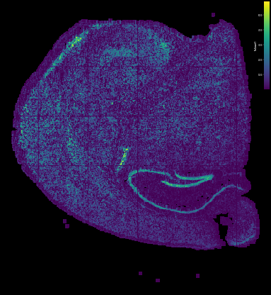
Read in example gem data, which holds mouse brain stereo-seq data from here.

gem = Gem.readin('../_static/data/example.gem.gz')

gem

	geneID	x	y	MIDCounts
0	Cr2	10059	14612	1
1	Cr2	6066	11227	3
2	Cr2	10521	11108	1
3	Cr2	8072	11782	3
4	Cr2	7891	16372	1
...	...	...	...	...
106663420	CAAA01147332.1	12756	17013	1
106663421	CAAA01147332.1	11907	12871	1
106663422	CAAA01147332.1	14707	4862	1
106663423	CAAA01147332.1	9787	5437	1
106663424	CAAA01147332.1	10471	15907	1

106663425 rows × 4 columns

preliminary understanding of your data

GEM saves spatial transcriptomics data, which can be easily understanding by seeing what it looks like.

gem.plot(color='nCount', bin_size=20)

None

[<Axes: >]

here you may focus on two points: 1. whether the spatial distributuion of the data is well decoded 2. how many features were captured in each square bin or DNB

extract data where tissue covered

Not all DNBs on the stereo-seq chip were covered by the tissue. An effective way for deleting non-related data is to use a mask, which is often a two dimensional numpy ndarray with tissue regions labeled as non-zero integer (see here). Once prepared a ready-to-use mask matrix, you can process as following:

import numpy as np
mask = np.loadtxt('../_static/data/example.transformed_mask.txt.gz')
mask.shape

(14451, 14248)

gem.img_shape

(14451, 14248)

gem = gem.mask(matrix=mask, return_offset=False, label_object=True)

now the gem data will be

gem.plot(color='nCount', bin_size=20)

None

[<Axes: >]

aggregate the data into cell/bin unit

After getting the effective data set, the next step is to determine how to group the nanometer-resolution DNB array into a analysis-ready unit, here always in two way: 1. group into square bin with equal width and height 2. group into putative cells

1. group into square bin

Square binning strategy do NOT consider any other informations like nucleus location and molecular homogeny. The only parameter in this step is bin_size, which specify how many DNBs in width and height should be grouped as a single bin unit. People can change this value based on the physical area of each bin and the captured features in each bin unit.

binning_gem = gem.binning(bin_size=20)
binning_gem

	geneID	x	y	label	MIDCounts
0	0610005C13Rik	5780	12540	16200	3
1	0610005C13Rik	5960	12760	14612	1
2	0610005C13Rik	5980	10700	28985	3
3	0610005C13Rik	6100	10240	32093	1
4	0610005C13Rik	6140	11420	23757	2
...	...	...	...	...	...
31798037	mt-Nd6	12880	8940	37309	2
31798038	mt-Nd6	12880	8960	37122	2
31798039	mt-Nd6	12880	9140	36185	1
31798040	mt-Nd6	12900	8640	39087	2
31798041	mt-Nd6	12900	8840	37995	3

31798042 rows × 5 columns

2. group into putative cells

Currently stereo-seq comprehend ssDNA stainning protocal, which stains the nucleus of cells on the same section. With the location of cell nucleus decoded, labeled with numpy mask file. And in the previous gem.mask process, we have labeled each DNB with their cell IDs by setting label_object=True.

gem

	geneID	x	y	MIDCounts	label
0	Cr2	8072	11782	3	20638
1	Cr2	7832	10872	1	27089
2	Cr2	6608	10674	1	28950
3	Cr2	9790	14297	2	3574
4	Cr2	6594	12299	2	17562
...	...	...	...	...	...
37759281	CAAA01147332.1	12231	11534	1	20817
37759282	CAAA01147332.1	10776	12505	2	14553
37759283	CAAA01147332.1	9810	10370	1	29920
37759284	CAAA01147332.1	10653	12974	1	11713
37759285	CAAA01147332.1	8062	11252	2	24214

37759286 rows × 5 columns

with cell ID labels, the gem file could be aggregated into cell-gene matrix as AnnData object

adata = gem.to_anndata()
adata

AnnData object with n_obs × n_vars = 41502 × 25288

the anndata object can be write into h5ad file and further used in clustering analysis

adata.write('../_static/data/example.h5ad')